FragFM: Hierarchical Framework for Efficient Molecule Generation via Fragment-Level Discrete Flow Matching

Lee, Joongwon; Kim, Seonghwan; Moon, Seokhyun; Kim, Hyunwoo; Kim, Woo Youn

FragFM: Hierarchical Framework for Efficient Molecule Generation via Fragment-Level Discrete Flow Matching

ICLR 2026

Joongwon Lee^1,*, Seonghwan Kim^1,2,*, Seokhyun Moon^1,*, Hyunwoo Kim^3,†, Woo Youn Kim^1,4,5,†

¹KAIST, Department of Chemistry ²KAIST, InnoCORE AI-CRED Institute ³Dongguk University, College of Pharmacy ⁴KAIST, Department of Data Science ⁵HITS

^*Equal Contribution ^†Corresponding Authors

Code arXiv Cite

BibTeX

@article{lee2025fragfm,
  title   = {FragFM: Hierarchical Framework for Efficient Molecule Generation via Fragment-Level Discrete Flow Matching},
  author  = {Lee, Joongwon and Kim, Seonghwan and Moon, Seokhyun and Kim, Hyunwoo and Kim, Woo Youn},
  journal = {arXiv preprint arXiv:2502.15805},
  year    = {2025}
}

Overview of the FragFM framework — **Overview.** **(a)** A coarse-to-fine autoencoder maps an atom-level graph G to a fragment-level graph 𝒢 and a latent z; discrete + continuous flows generate (𝒢, z) while f_θ picks fragments from a stochastic bag ℬ. **(b)** The decoder reconstructs atom-level edges via Blossom matching.

Abstract

We introduce FragFM, a novel hierarchical framework via fragment-level discrete flow matching for efficient molecular graph generation. FragFM generates molecules at the fragment level, leveraging a coarse-to-fine autoencoder to reconstruct details at the atom level. Together with a stochastic fragment bag strategy to effectively handle a large fragment space, our framework enables more efficient, scalable molecular generation. We demonstrate that our fragment-based approach achieves better property control than the atom-based method and additional flexibility through conditioning the fragment bag. We also propose a Natural Product Generation benchmark (NPGen) to evaluate the ability of modern molecular graph generative models to generate natural product-like molecules. Since natural products are biologically prevalidated and differ from typical drug-like molecules, our benchmark provides a more challenging yet meaningful evaluation relevant to drug discovery. We conduct a comparative study of FragFM against various models on diverse molecular generation benchmarks, including NPGen, demonstrating superior performance. The results highlight the potential of fragment-based generative modeling for large-scale, property-aware molecular design, paving the way for more efficient exploration of chemical space.

Contributions

Molecular graph generative models

Atom-based

Chemically implausible
Poor scaling
Low controllability

Fragment-based

Limited fragment library
Poor scaling
Hard to recover whole graph

FragFM

ours

The first fragment-level graph flow matching that explores meaningful chemical space at scale.

What FragFM solves

Challenge

Large fragment vocabulary

FragFM

Stochastic fragment bag

Challenge

Generalizing to new fragments

FragFM

GNN fragment embedding

Challenge

One-to-many atom mapping

FragFM

Coarse-to-fine autoencoder

What FragFM shows

Higher performance

Scalability

Better conditioning

Method

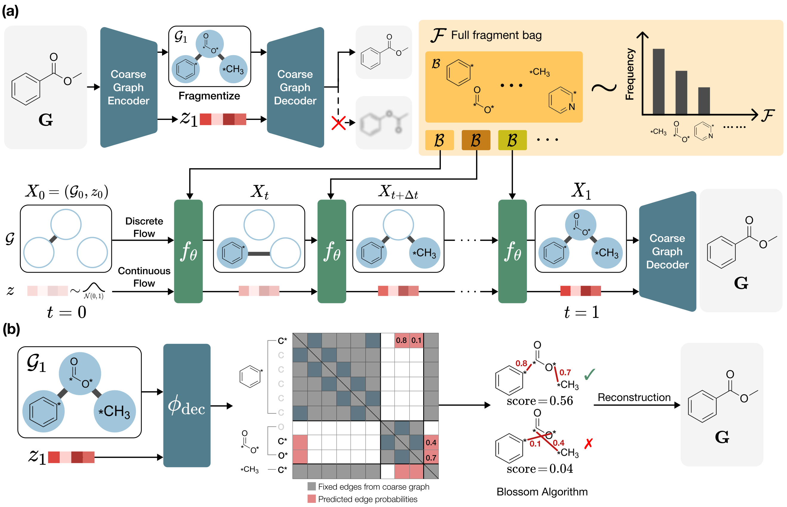
FragFM rests on two ideas. (i) A coarse-to-fine autoencoder compresses an atom-level graph G into a much smaller fragment-level graph 𝒢 plus a single continuous latent z that carries the atom-level connectivity. (ii) On that fragment-level graph, discrete flow matching (DFM) generates fragment types; to make the huge fragment vocabulary tractable, training and sampling are restricted to a stochastic fragment bag 𝓑 ⊂ 𝓕, optimized with an Info-NCE objective.

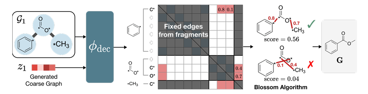
Coarse-to-Fine Autoencoder

The encoder first applies a deterministic fragmentation rule (BRICS) to split G into fragments, then a graph neural network φ_enc encodes both into a latent z that remembers which atoms were bonded across fragment cuts. The decoder φ_dec scores candidate inter-fragment atom pairs and feeds those scores into the Blossom matching algorithm to recover exact atom-level edges E.

Reconstruction accuracy — test set (%)

Dataset	Bond	Graph
MOSES	99.99	99.93
GuacaMol	99.98	99.42
ZINC250k	99.64	98.71
NPGen	99.71	97.43

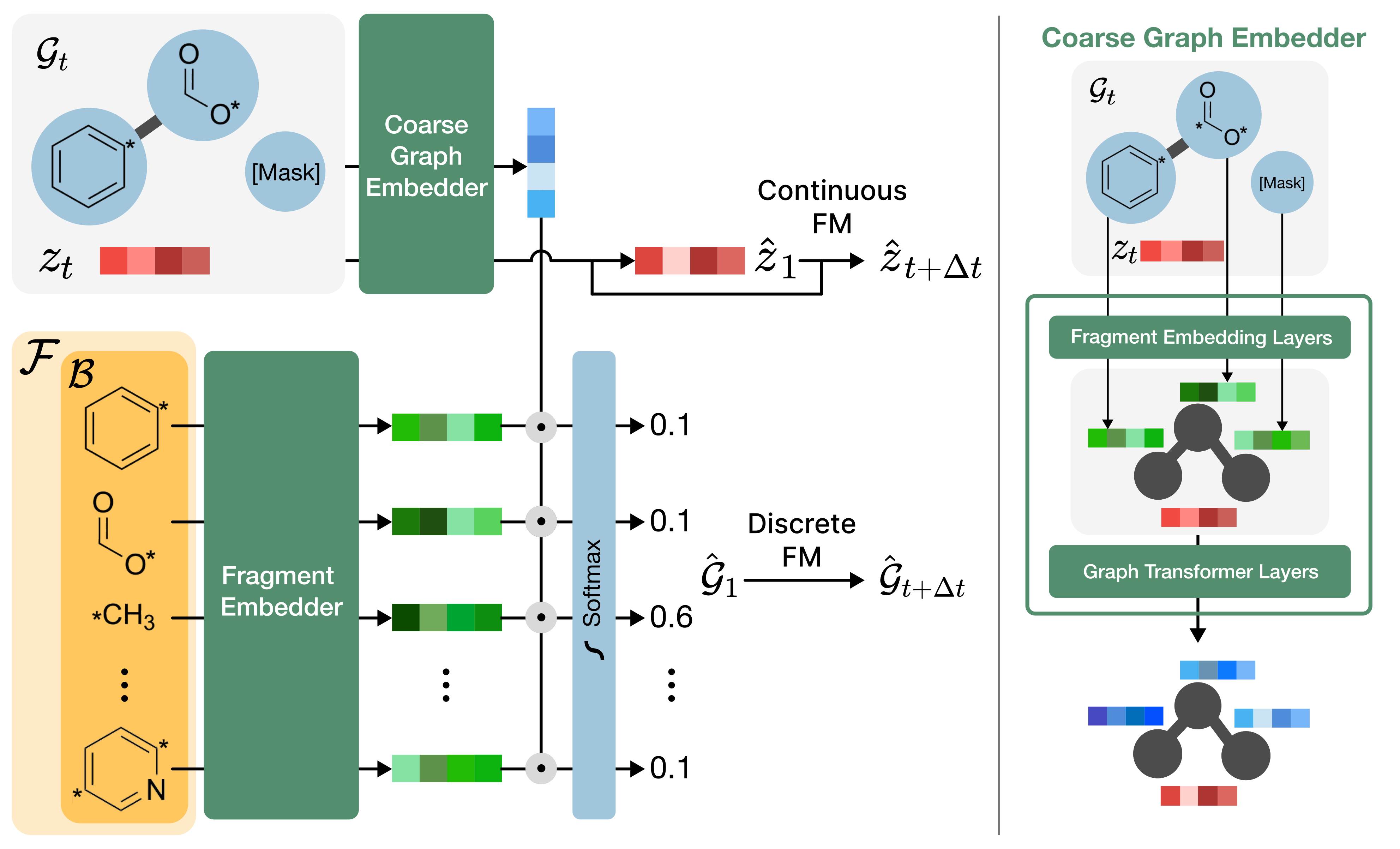
$$ \textbf{Encoder:}\;\; \mathbf{G}\xrightarrow{\text{Rule}}\mathcal{G},\quad (\mathbf{G},\mathcal{G})\xrightarrow{\phi_{\text{enc}}} z $$ $$ \textbf{Decoder:}\;\; (\mathcal{G},z)\xrightarrow{\phi_{\text{dec}}}\text{score}\xrightarrow{\text{Blossom}}\mathbf{E} $$

reconstruction the fragment-level graph + latent z is a near-lossless compression, achieving >99% bond-level accuracy across all four benchmarks (see table).

Fragment-Level Flow Matching with Stochastic Bag

On the coarse graph X = (𝒢, z), FragFM runs discrete flow matching (DFM) over fragment types and continuous flow matching over the latent. To avoid a softmax over the full fragment vocabulary 𝓕 (which can exceed 10⁵ fragments), each step samples a bag 𝓑 ⊂ 𝓕 of size N and restricts the denoiser's softmax to 𝓑. A neural density-ratio estimator f_θ(X_t, x) is trained with an Info-NCE loss against one positive + N−1 negative fragments:

$$ \mathcal{L}(\theta) = -\,\mathbb{E}_{\mathcal{B}}\!\left[\,\log \frac{f_{\theta}(X_t,\,x^{+})} {\displaystyle\sum_{y\in\mathcal{B}} f_{\theta}(X_t,\,y)} \right] $$

Info-NCE pushes the positive fragment x⁺ above N−1 sampled negatives inside 𝓑, so f_θ approximates the density ratio p_1|t(x|X_t) / p₁(x).

scaling training and sampling cost is O(N) per step, independent of |𝓕| — decoupling model cost from vocabulary size.

At inference, the trained f_θ defines an in-bag posterior over 𝓑, which the sampler integrates into a one-step Euler transition kernel:

$$ p^{\theta}_{1|t,\mathcal{B}}(x_1 \mid X_t, \mathcal{B}) = \frac{\mathbf{1}_{\mathcal{B}}(x_1)\, f_{\theta}(X_t, x_1)} {\sum_{y\in\mathcal{B}} f_{\theta}(X_t, y)} $$ $$ p^{\theta}_{t+\Delta t|t}(x_{t+\Delta t}\mid X_t, \mathcal{B}) = \mathbb{E}_{x_1\sim p^{\theta}_{1|t,\mathcal{B}}} \!\left[\, p_{t+\Delta t|t}(x_{t+\Delta t}\mid X_t, x_1)\,\right] $$

posterior softmax over the sampled bag 𝓑 — never over the full vocabulary 𝓕.

kernel a standard DFM Euler step; as N→|𝓕| it converges to the exact transition kernel, so small Δt + moderate N suffices in practice.

Parameterization of fragment embedder and prediction head f_theta — **Parameterization of *f_θ*.** (left) Each fragment in 𝓑 is embedded by a GNN fragment embedder; coarse-graph nodes are mapped to fixed-size vectors; *f_θ(X_t, x)* is their inner product. (right) The coarse-graph embedder first vectorizes each node, then processes the whole graph with a graph transformer. Shared fragment embeddings let FragFM generalize to fragments unseen at training.

Benchmarks

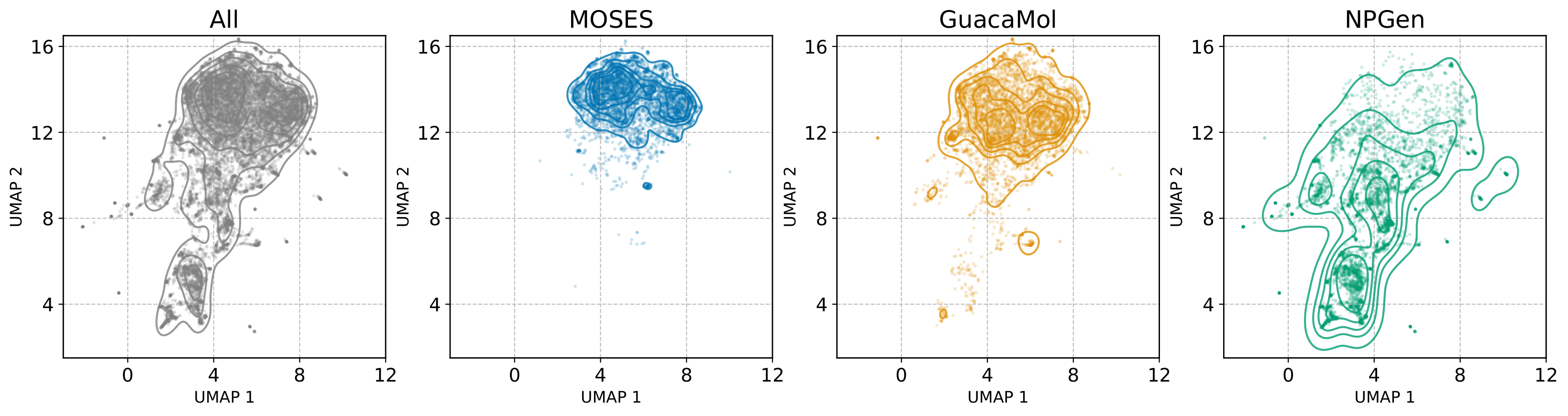
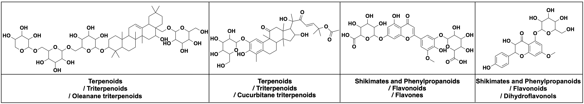
NPGen — A Natural Product Benchmark

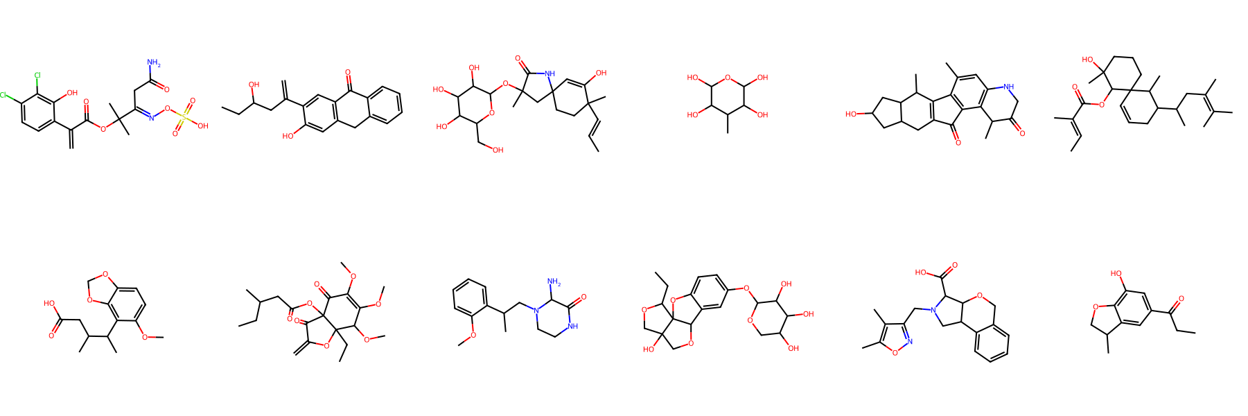
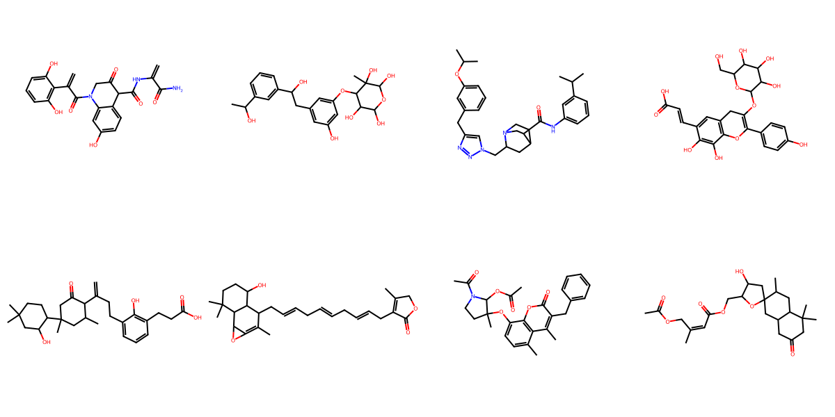
658,566 natural products from COCONUT, average 35.0 heavy atoms (vs. 21.7 MOSES, 27.9 GuacaMol). Evaluation adds NP-likeness and NP-Classifier divergences that reflect biological functionality rather than saturated distributional overlap.

UMAP of MOSES, GuacaMol, and NPGen — **Distinct chemical space.** UMAP of 5k samples per dataset.

**Representative NPGen molecules** with NP-Classifier pathway/superclass/class annotations.

Quantitative Results

FragFM is a graph generative model, evaluated against atom- and fragment-level graph baselines on four standard molecular-generation benchmarks — matching or setting SOTA across all of them. autoregressive / sequence and one-shot diffusion / flow baselines are shown for context. Bold = best; underline = second-best.

MOSES — 25k generated molecules

Model	Valid ↑	Unique ↑	Novel ↑	Filters ↑	FCD ↓	SNN ↑
Training set	100.0	100.0	–	100.0	0.48	0.59
GraphINVENT	96.4	99.8	–	95.0	1.22	0.54
JT-VAE	100.0	100.0	99.9	97.8	1.00	0.53
DiGress	85.7	100.0	95.0	97.1	1.19	0.52
DisCo	88.3	100.0	97.7	95.6	1.44	0.50
Cometh	90.5	100.0	96.4	97.2	1.44	0.51
Cometh-PC	90.5	99.9	92.6	99.1	1.27	0.54
DeFoG	92.8	99.9	92.1	98.9	1.95	0.55
FragFM (ours)	99.8	100.0	87.1	99.1	0.58	0.56

GuacaMol — 10k generated molecules

Model	Val. ↑	V.U. ↑	V.U.N. ↑	KL Div. ↑	FCD ↑
Training set	100.0	100.0	–	99.9	92.8
MCTS	100.0	100.0	95.4	82.2	1.5
DiGress	85.2	85.2	85.1	92.9	68.0
DisCo	86.6	86.6	86.5	92.6	59.7
Cometh	94.4	94.4	93.5	94.1	67.4
Cometh-PC	98.9	98.9	97.6	96.7	72.7
DeFoG	99.0	99.0	97.9	97.7	73.8
FragFM (ours)	99.7	99.3	95.0	97.4	85.8

ZINC250k — 25k generated molecules

Model	Valid ↑	NSPDK ↓	FCD ↓
Training set	–	0.0001	0.062
GraphAF	67.92	0.0432	16.128
GraphDF	89.72	0.1737	33.899
MolHF	94.75	0.0709	22.230
GDSS	97.12	0.0192	14.032
GSDM	92.57	0.0168	12.435
GruM	98.32	0.0023	2.235
SwinGNN	86.16	0.0047	4.398
DiGress	94.98	0.0021	3.482
GGFlow	99.63	0.0010	1.455
FragFM (ours)	99.81	0.0002	0.630

NPGen — 30k generated natural-product-like molecules

Model	Val. ↑	Unique ↑	Novel ↑	NP Score KL Div. ↓	NP Class KL Div. ↓			FCD ↓
Model	Val. ↑	Unique ↑	Novel ↑	NP Score KL Div. ↓	Pathway	Superclass	Class	FCD ↓
Training set	100.0	100.0	–	0.0006	0.0002	0.0028	0.0094	0.01
GraphAF	79.1	63.6	95.6	0.8546	0.9713	3.3907	6.6905	25.11
JT-VAE	100.0	97.2	99.5	0.5437	0.1055	1.2895	2.5645	4.07
HierVAE	100.0	81.5	97.7	0.3021	0.4230	0.5771	1.4073	8.95
DiGress	85.4	99.7	99.9	0.1957	0.0229	0.3370	1.0309	2.05
DeFoG	85.9	98.4	99.2	0.1550	0.1252	0.4134	1.3597	4.46
FragFM (ours)	98.0	99.0	95.4	0.0374	0.0196	0.1482	0.3570	1.34

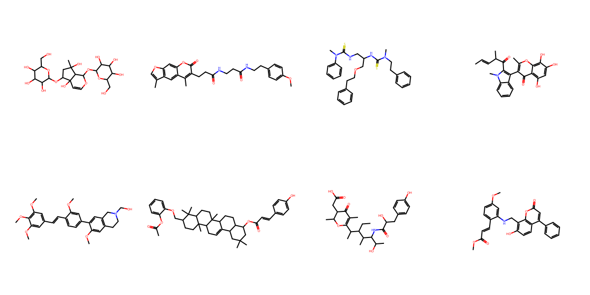
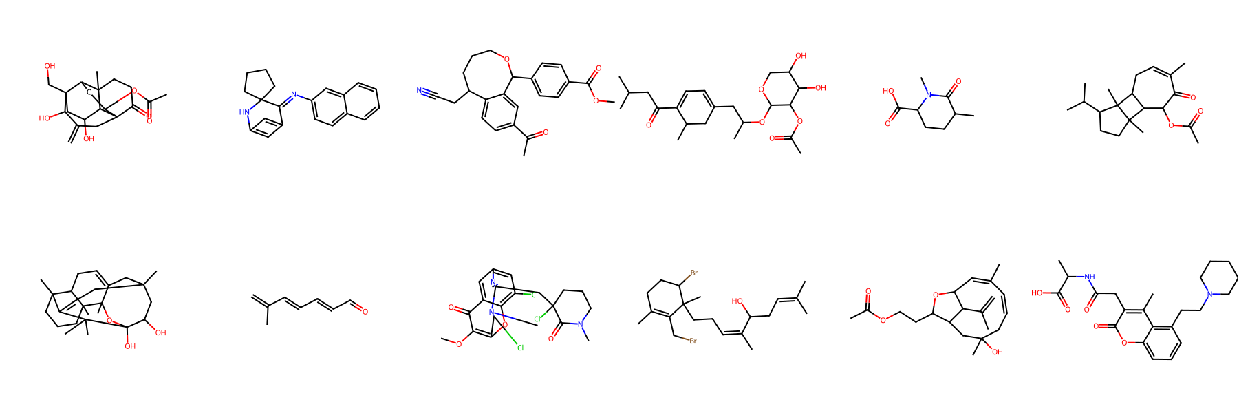
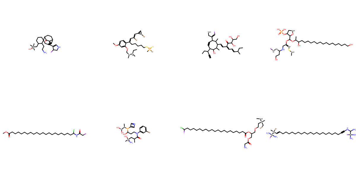
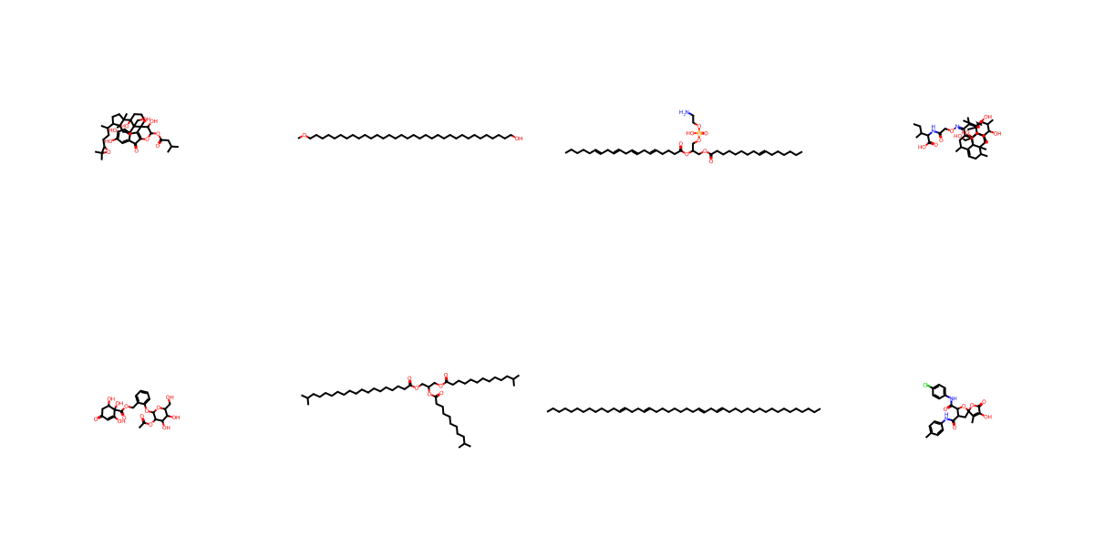
NPGen Samples Across Models

Click a model to browse its NPGen samples — across small (≤30 heavy atoms) and large (31–60) molecules.

Up to 30 heavy atoms

31–60 heavy atoms

Up to 30 heavy atoms

31–60 heavy atoms

Up to 30 heavy atoms

31–60 heavy atoms

Up to 30 heavy atoms

31–60 heavy atoms

Up to 30 heavy atoms

31–60 heavy atoms

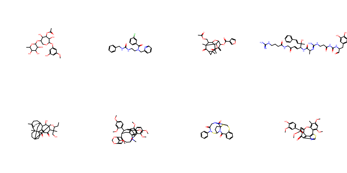
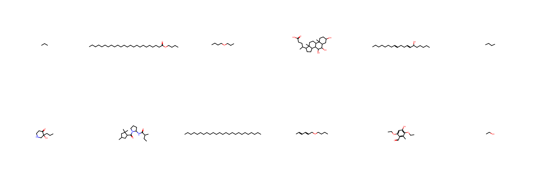
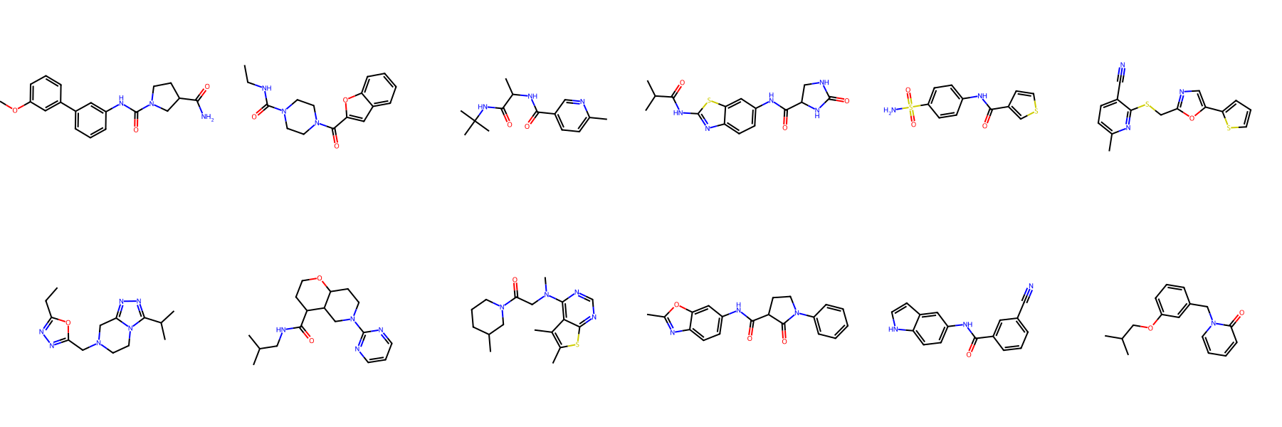
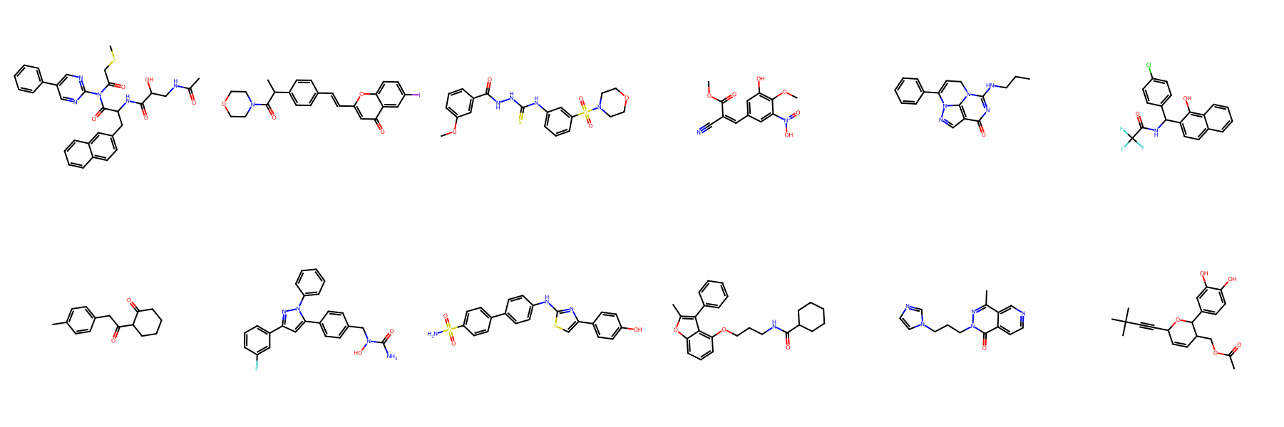
Generated Sample Gallery

Random valid molecules generated by FragFM on the standard drug-like benchmarks MOSES and GuacaMol.

FragFM-generated molecules on MOSES (drug-like small molecules) — MOSES

FragFM-generated molecules on GuacaMol — GuacaMol

Conditional Generation

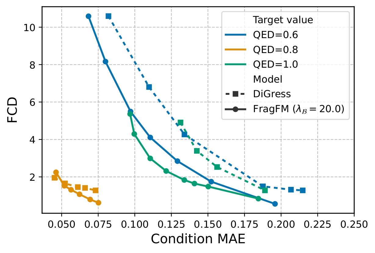
Property-Controlled Generation

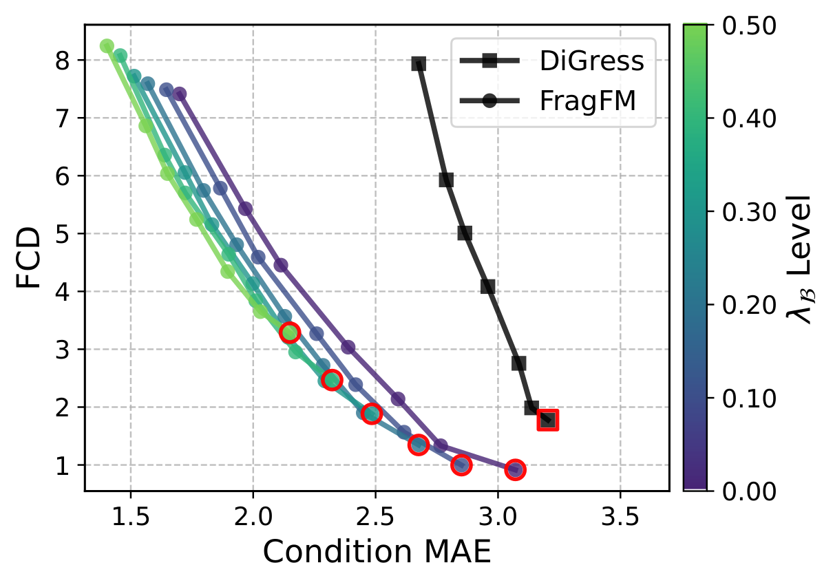
FragFM exposes two guidance knobs: standard classifier guidance λ_X that pulls the flow trajectory toward a target property c, and fragment-bag reweighting λ_𝓑 that biases the fragment bag 𝓑 itself — up-weighting fragments whose predicted property matches the target.

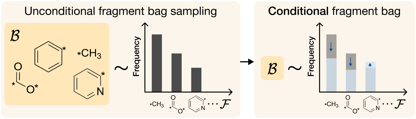
Unconditional vs conditional fragment bag sampling — **Fragment-bag guidance (*λ_𝓑*).** At inference, the fragment bag 𝓑 is reweighted by a fragment-level property predictor: fragments helpful for target c are amplified, others suppressed — yielding the conditional bag *𝓑^c*.

Both knobs drop out of a single Bayes decomposition of the property-conditioned in-bag transition kernel:

$$ p(X_{t+\Delta t}\mid X_t,\mathcal{B}^{c},c) \;=\; \underbrace{\;p(X_{t+\Delta t}\mid X_t,\mathcal{B}^{c})\;}_{\color{#4f46e5}{\mathcal{B}^{c}\text{ steered by }\lambda_{\mathcal{B}}}} \;\cdot\; \underbrace{\;\frac{p(c\mid X_{t+\Delta t},X_t,\mathcal{B}^{c})}{p(c\mid X_t,\mathcal{B}^{c})}\;}_{\color{#4f46e5}{\text{steered by }\lambda_X}} $$

λ_𝓑 biases the bag 𝓑^c toward fragments whose predicted property matches c.

λ_X is the classifier-guidance strength on the in-bag transition kernel.

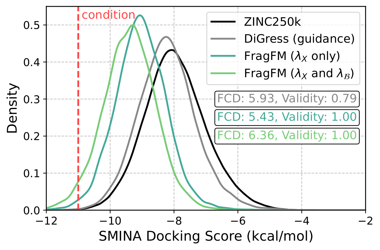
On the hard JAK2 docking-score task (top 0.08% of ZINC250k), bag guidance alone reaches the target while DiGress collapses in validity.

QED MAE-FCD — **QED.** MAE–FCD across target values.

JAK2 docking KDE — **JAK2 KDE.** Only FragFM reaches −11.0 kcal/mol.

Bag guidance effect — **Bag guidance.** *λ_𝓑* shifts MAE–FCD curves; red = bag-only (*λ_X*=0).

Synthesizability via Fragment-Bag Swap

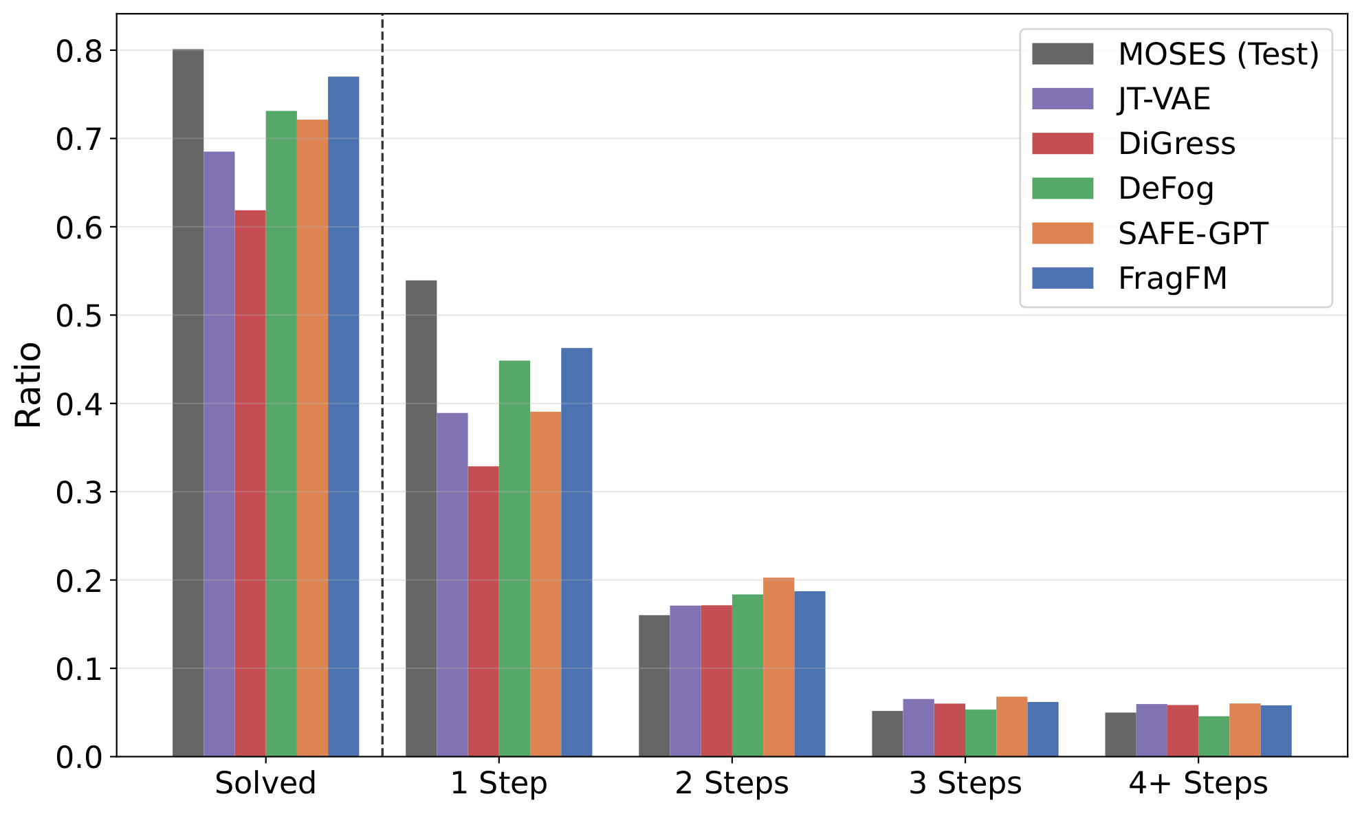
AIZynthFinder retrosynthesis on 25k MOSES samples: FragFM reaches 77% solved, close to the MOSES test set (80%). Swapping the fragment bag to fragments drawn from solved (synthesizable) molecules — no retraining — pushes it to 85%, exceeding the dataset itself.

Each glyph is a chemical fragment; FragFM assembles fragments into molecules. Restricting the bag to a subset — fragments drawn only from AIZynth-solved molecules (faded glyphs are filtered out) — lifts the synthesizable rate from 77% → 85% with no retraining.

AIZynthFinder	Solved ↑	1 step	2 steps	3 steps	4+ steps
MOSES (test set)	80.1	53.9	16.0	5.17	5.0
FragFM	77.0	46.3	18.7	6.2	5.8
FragFM · solved bag	85.0	52.3	20.7	6.6	5.4

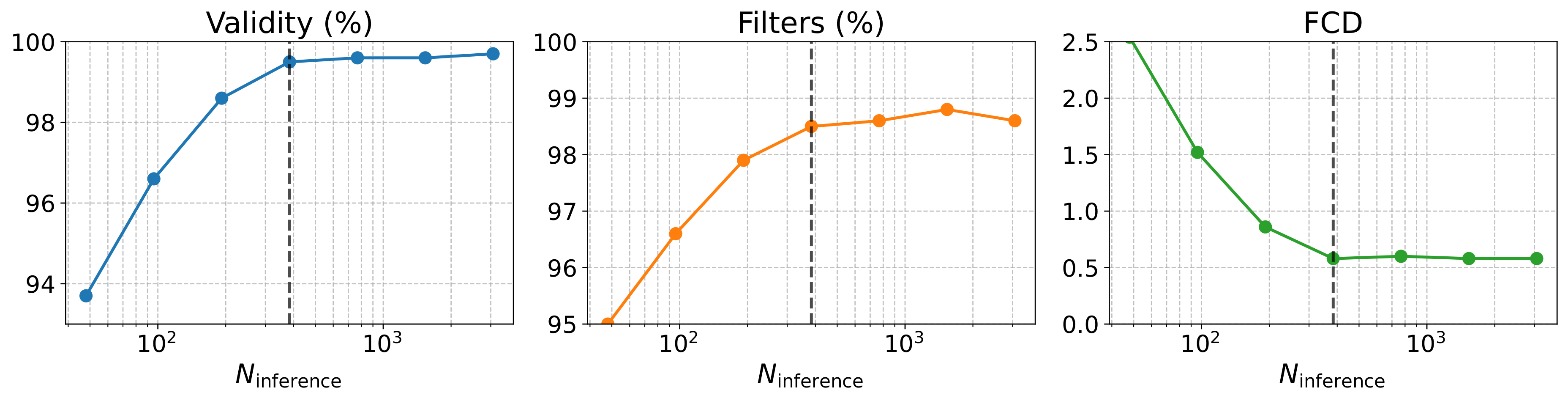
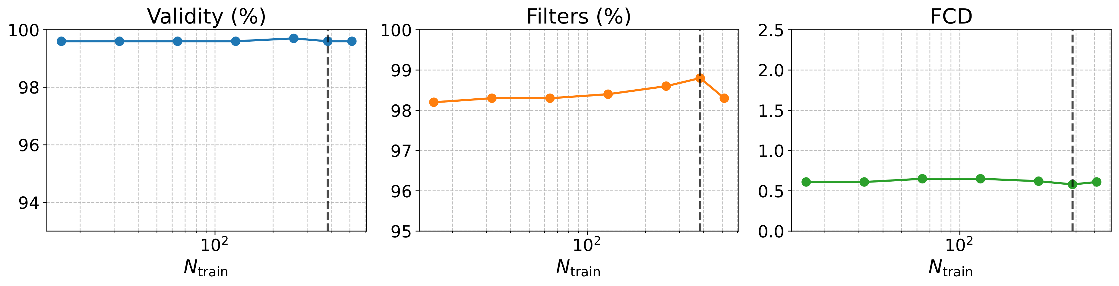
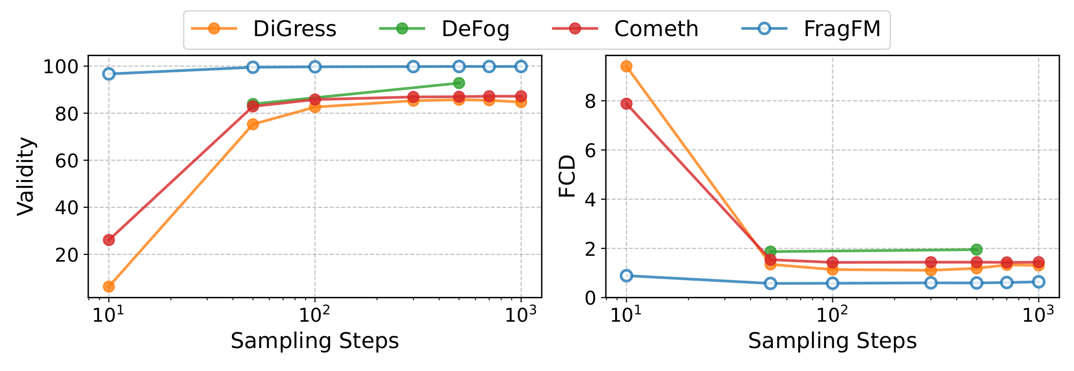
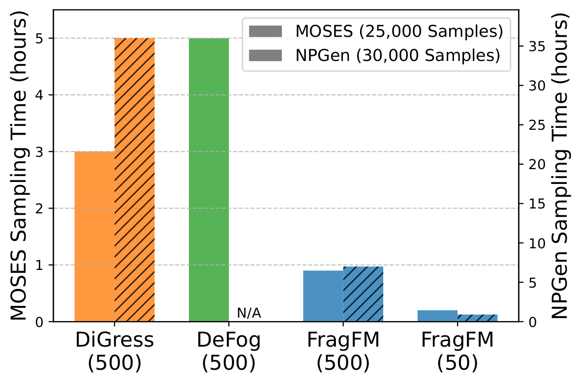
Fraction (%) of 25k MOSES generations solved by AIZynthFinder, split by route length.

AIZynthFinder synthesis-step distribution across models — **Baseline comparison.** FragFM has the lowest unsolved rate among learned generators.

Scalability

Denoising at the fragment level — not over individual atoms — keeps validity above 95% and FCD below 1.0 even under aggressive step reduction, with ~5× faster wall-clock time than DiGress on NPGen.

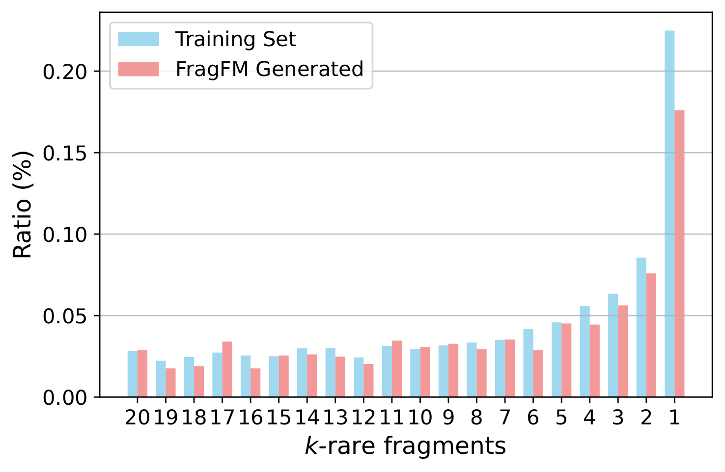
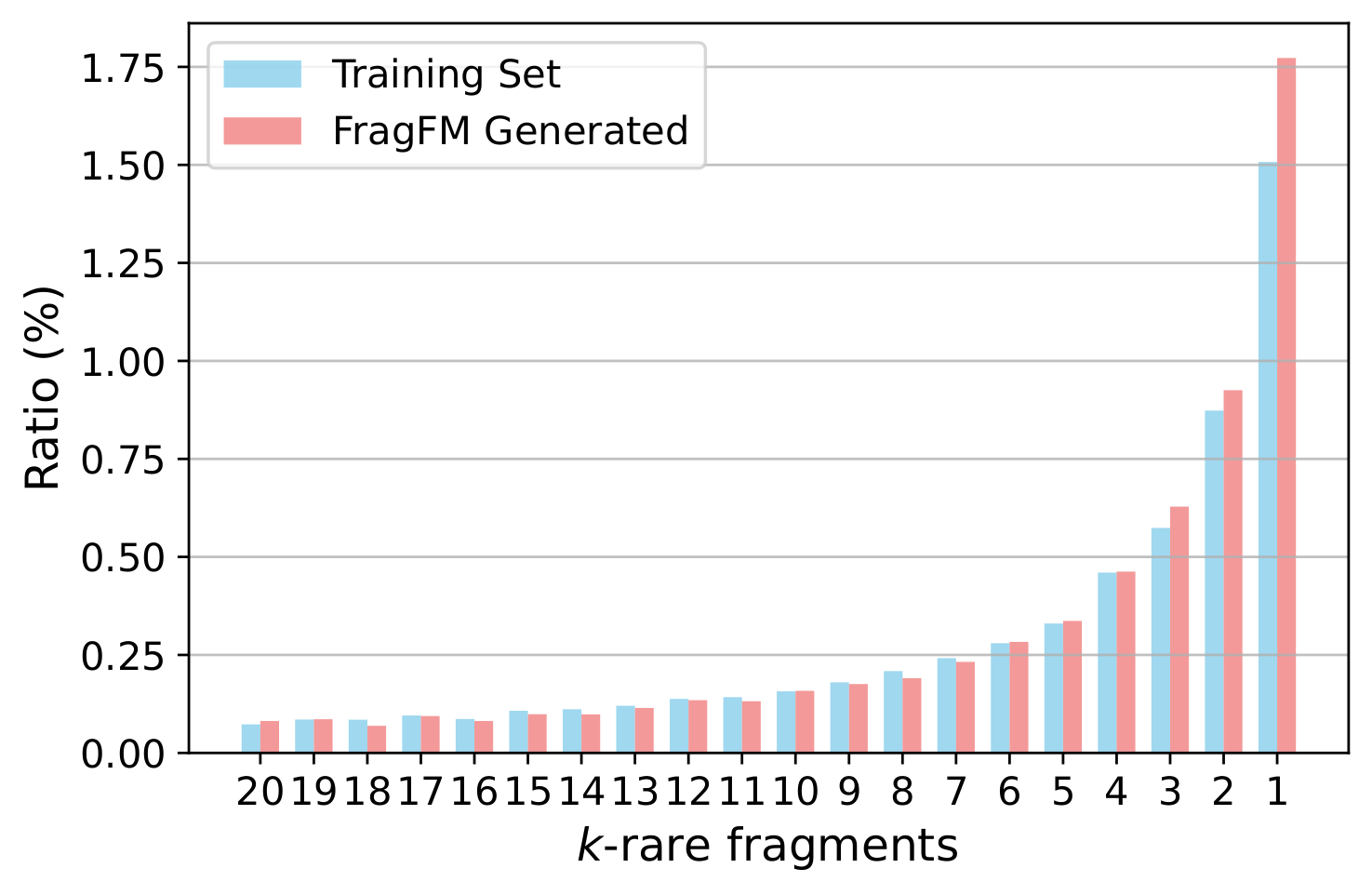
Sampling step ablation — **Step ablation.** Atom-based baselines collapse as steps shrink; FragFM holds up.

Wall-clock sampling time — **Wall-clock time.** MOSES and NPGen; (·) = sampling steps.

Additional Results

Ablations over the fragmentation rule, sampling temperature, fragment-bag size, and how well FragFM recovers rare fragments.

(a) Robustness to fragmentation rule — BRICS vs RECAP vs rBRICS, no retraining

Swapping BRICS for RECAP or rBRICS — keeping all hyperparameters fixed — barely moves the quality metrics. The framework is not tied to a specific fragmentation scheme.

Rule	MOSES						ZINC250k
Rule	Valid ↑	Unique ↑	Novel ↑	Filters ↑	FCD ↓	SNN ↑	Valid ↑	NSPDK ↓	FCD ↓
Training set	100.0	100.0	–	100.0	0.48	0.59	100.0	0.0001	0.062
BRICS (default)	99.8	100.0	87.1	99.1	0.58	0.56	99.81	0.0002	0.630
RECAP	99.8	99.9	83.6	99.3	0.56	0.57	99.66	0.0003	0.580
rBRICS	99.8	100.0	88.5	98.7	0.58	0.56	99.79	0.0003	0.563

(b) Temperature scaling on MOSES — quality–novelty trade-off via 𝒯_pred and 𝒯_bag

Two knobs shift the quality–novelty frontier: 𝒯_pred on the denoiser's softmax and 𝒯_bag on fragment-bag sampling. Raising 𝒯_bag pushes Novel and Scaf up at a small FCD cost.

𝒯_pred	𝒯_bag	Valid ↑	Unique ↑	Novel ↑	Filters ↑	FCD ↓	SNN ↑	Scaf ↑
1.0	1.0	99.8	100.0	87.1	99.1	0.58	0.56	10.9
1.0	1.5	99.2	100.0	94.2	98.3	0.90	0.52	13.5
1.5	1.0	99.7	100.0	88.6	98.8	0.88	0.54	11.0
1.5	1.5	99.2	100.0	94.5	98.3	0.91	0.51	13.1

(c) Effect of fragment-bag size on MOSES — inference-time and training-time bag size ablations

Performance is largely saturated above the default (N = 384, dashed line). Inference-time is more sensitive than training-time — a moderate bag suffices for training, while inference quality continues to improve with larger N_inference.

Effect of inference-time fragment-bag size — **(a) Inference-time bag size** (with N_train = 384). Validity / Filters / FCD vs N_inference on log-scale.

Effect of training-time fragment-bag size — **(b) Training-time bag size** (with N_inference = 384). The black dashed line marks the default FragFM configuration.

(d) Long-tail fragment recovery — 20 rarest fragments per dataset, training vs FragFM ratios

For each dataset, the 20 rarest fragments (k = 1 is the rarest) are plotted. FragFM-generated ratios closely track the training-set ratios — even for fragments that appear only a handful of times in training.

Long-tail fragment recovery on MOSES — **(a) MOSES**

Long-tail fragment recovery on GuacaMol — **(b) GuacaMol**

Long-tail fragment recovery on NPGen — **(c) NPGen**